Excel Data Validation lists are a great way to

expedite data entry
ensure consistent data entry
reject undesirable information

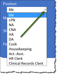
One of the few and far between shortcoming of Data Validation lists is the fact that with long lists, they have to exist somewhere in the workbook. The existing list supplies the entries displayed when the dropdown list is activated.

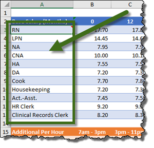
The existence of the list is not in and of itself an issue, maintaining the list (adding and removing items from the list) and having those changes propagate to the Data Validation dropdown is the problem. Over the years there have been some very creative solutions developed by some truly ingenious people. The process below appears to be the most straight-forward and effective solution developed.

Step 1: Create a list

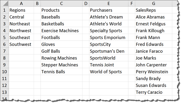
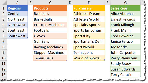
If you are providing lists for several Data Validation dropdown lists, a best practice is to create a separate sheet (called “DDLists”, perhaps) and localize all of the lists to this sheet, one list per column.

Step 2: Convert each list into an official Excel Data Table

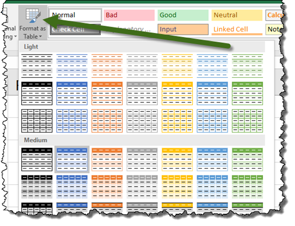
Select a list (perform this step separately for each list) and navigate to the Home ribbon. In the Styles group select Format as Table. Select the color scheme of your choice.

Repeat this process for each list on the sheet.

Step 3: Name each data table

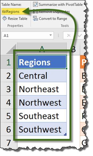
Selecting each table (one at a time), select the Table Tools – Design ribbon. In the Properties group (far left side of ribbon), change the table name to something memorable; i.e. “tblRegions”.

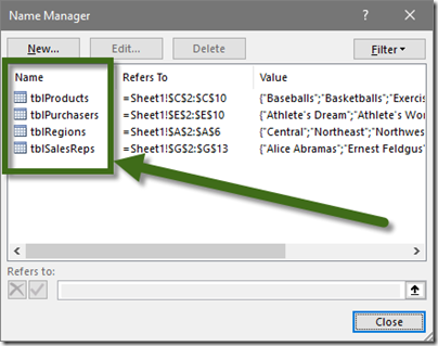
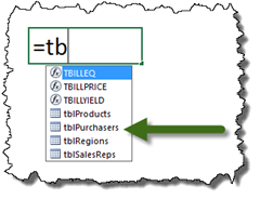
If the tables are prefaced with something like “tbl”, “t”, or “tb”, all of the tables will appear grouped together in the Name Manager and when using Excel AutoComplete feature during hand-typed formulas.

Step 4: Create the Data Validation rule

Select the cell where the dropdown list is to appear. From the Data ribbon, in the Data Tools group, select Data Validation.

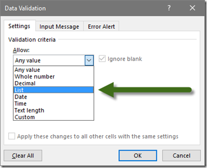
In the Data Validation dialog box, from the Allow dropdown, select List.

In the Source field, type the following formula:

=INDIRECT(“tblRegions[Regions]”)

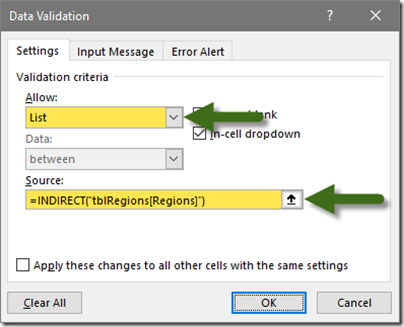
The parts of the formula are as follows:

=INDIRECT(“tblRegions[Regions]“)

INDIRECT è The function used to retrieve the list

tblRegions è The name of the Data Table

[Regions] è The name of the column holding the list

**** IMPORTANT ****

Ensure you enclose the table and column name in double quotes

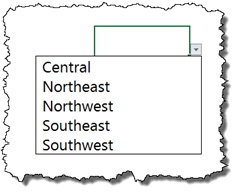
A dropdown arrow will appear allowing for list entries to be selected.

The Best Part

If an new entry has to be included in a list, simply add the entry to the bottom of the list. The data table will automatically expand to absorb the new item.

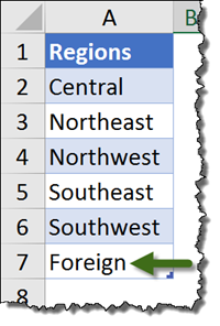
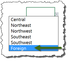
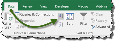
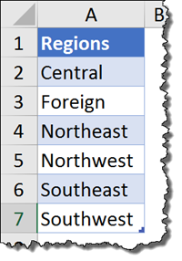
If you wish the list to be sorted, click on any item in the list. From the Data ribbon, in the Sort & Filter group, select Ascending Sort.

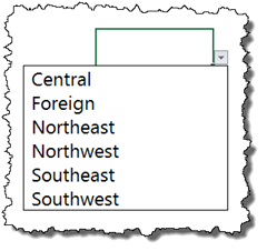
The result will be a sorted list.

BONUS TIP

If you have several single column lists (like the ones above), and you wish to keep all of those lists sorted, the VBA code below will sort the lists after all of the modifications are made to the lists. Make your changes to the list(s); upon leaving the sheet, the VBA code will run and loop through all of the tables on that sheet, sorting each list alphabetically in ascending order.

Copy and paste the below code to the code sheet of the sheet holding all of the lists.

VBA CODE

Private Sub Worksheet_Deactivate()

Dim FirstCell As String
Dim tbl As ListObject

For Each tbl In ActiveSheet.ListObjects

        tbl.DataBodyRange.Cells(1, 1).Select

        FirstCell = ActiveCell.Address

            With tbl.Sort
                .SortFields.Clear
            End With

            With tbl.Sort
                .SortFields.Add Key:=Range(FirstCell), _
                 SortOn:=xlSortOnValues, _
                 Order:=xlAscending, _
                 DataOption:=xlSortNormal
            End With

            With tbl.Sort
                .Header = xlYes
                .MatchCase = False
                .Orientation = xlTopToBottom
                .SortMethod = xlPinYin
                .Apply
            End With

    Next tbl

End Sub