Excel – Create Named Ranges Quickly and Use Retroactively

Excel Named Ranges are a great way to turn ugly, confusing formulas into easy to read statements.  Consider the following formula:

    =($J$44 – $M$213) * $H$16   

Without any context given to the formula, the viewer has no idea what this is supposed to produce.  The only obvious logic is that there is some subtraction and multiplication taking place.  But consider this modified version of the same formula:

    =(OrderSubTotal – Discount) * NYStateTax   

Even without context, the formula is self explanatory; “Take the order subtotal and deduct the discount, then multiply the result by the New York state sales tax.”  Named ranges make any formula easier to read.

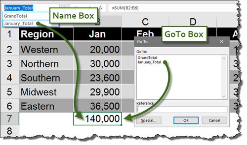
In addition to easier to read formulas, named ranges, when referenced from the Name Box or GoTo dialog box, can navigate the user to the named range.

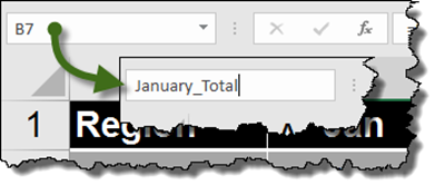
Creating the named range is as simple as selecting a cell and typing the desired name into the Name Box.

Although this is a great feature, if you have many named ranges you wish to use, creating each one separately can be a bit of a chore.  Luckily, Excel has a way to expedite the process.

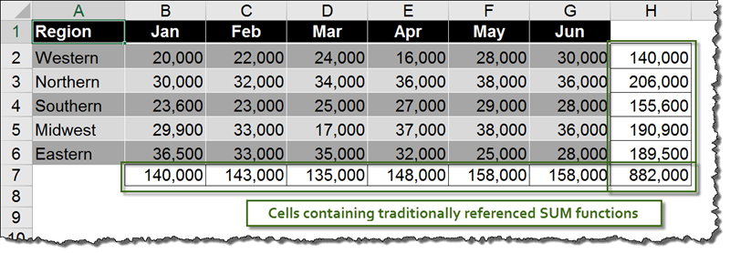
Take the following table of sales, for example:

The user would like to create a named range for each month (i.e. “JAN” would be defined as cells B2:B6) and a named range for each region (i.e. “Southern” would be defined as cells B4:G4.)

To create all of the month and region named ranges in a single operation,

Step 1:

Highlight all of the cells containing titles and data (i.e. A1:G6).

Step 2:

From the Formulas ribbon, in the Defined Names group, select Create from Selection.

Step 3:

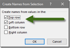
In the Defined Names from Selection dialog box, select Top row and Left column.  This will read the titles in column A and row 1 and assign those names to cells in the adjacent column and row cells.

Step 4:

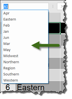
Select the Name Box dropdown to verify that all of the named ranges have been created.

Applying the Names Retroactively

Using named ranges in formulas makes formulas easier to read; but what if the formulas were created BEFORE the named ranges existed?  If the spreadsheet has formulas that references cells in the traditional manner, but those cells now have nice, useful names, there is a way to rewrite all of those formulas to use the names as if they existed from the beginning.

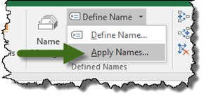
To “rewrite” all of the formulas to use the new named ranges, from the Formulas ribbon, in the Defined Names group, select the small down arrow to the right of Define Name.

Select Apply Names…

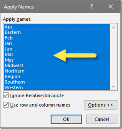
In the Apply Names dialog box, select any or all of the defined names that you wish to retroactively apply to existing formulas.  Click OK when finished.

Observe the original formulas in their new, easy to read format.